Phase plane
The phase plane draws trajectories of a system with two or more states against two of them, with the direction field, the nullclines and the fixed points. Choose Phase in the View panel.
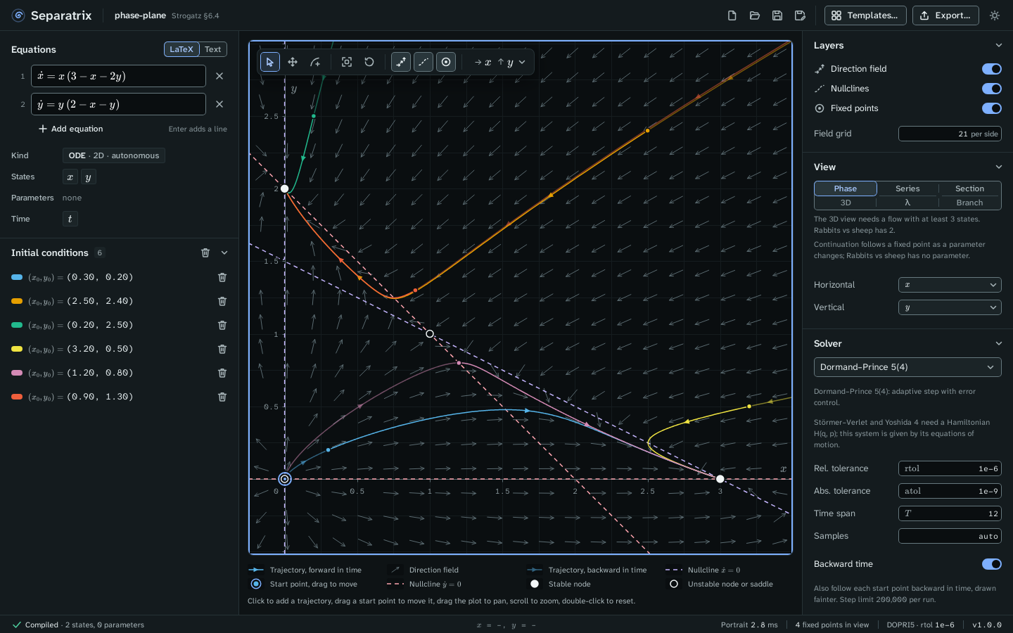
Example project: phase-plane.sepx, the rabbits-versus-sheep model of Strogatz §6.4. The fixed point at (0, 0) is unstable, (0, 2) and (3, 0) are stable nodes, and (1, 1) is a saddle, as the Strogatz gate checks.
Read the plot
| Mark | Meaning |
|---|---|
| Solid line with arrows | A trajectory, forward in time. |
| Fainter line | The same trajectory backward in time, when Backward time is on in the Solver panel. |
| Ringed dot | A start point. Drag it to move the trajectory. |
| Short arrows | The direction field, with arrows of normalized length. |
| Dashed lines | The nullclines, where ẋ = 0 or ẏ = 0. Each has its own color, named in the legend. |
| Filled circle | A stable fixed point. |
| Open circle | An unstable fixed point. |
The legend under the plot names every mark that is on screen. The status bar shows the pointer's coordinates and how many fixed points are in view.
Work with trajectories
- Click the plot to add a trajectory that starts there.
- Drag a start point to move it.
- Click a trajectory to select it. The Trajectories panel shows its start state, end state and the solver's step counts. Press Delete to remove it, or Escape to deselect it.
- Click the eye icon in the Trajectories panel to hide a trajectory without deleting it.
The toolbar in the top left corner of the plot has three tools: Select drags start points, Pan drags the plot, and Add trajectory adds a start point on each click. Its other buttons are Zoom to fit the trajectories, Reset view, and switches for the direction field, the nullclines and the fixed points.
Read the fixed points
The Fixed points panel lists every fixed point in view with its type (stable node, saddle, unstable spiral, center and so on) and its eigenvalues. Click a row or a fixed point on the plot to select it. Show eigenvectors draws a line along each real eigenvector, with arrows that point in for a stable direction and out for an unstable one.
Choose the axes
A system with more than two states shows two of them at a time. Choose the states in the Horizontal and Vertical menus of the View panel, or in the axes menu at the right end of the plot's toolbar. The other states are held at the values under Field slice for the direction field and the nullclines. Trajectories always use every state.
The field of a nonautonomous system, one with t on the right-hand side, changes with time. For
such a system, the field is drawn at Field at time under Field slice, and fixed points
are not searched.
Change the layers
The Layers panel switches the direction field, the nullclines and the fixed points on and off. Field grid sets the number of arrows per side, from 2 to 200.