Time series

The time series view plots a state against time, t for a flow or n for a map, for every trajectory. Choose Series in the View panel.

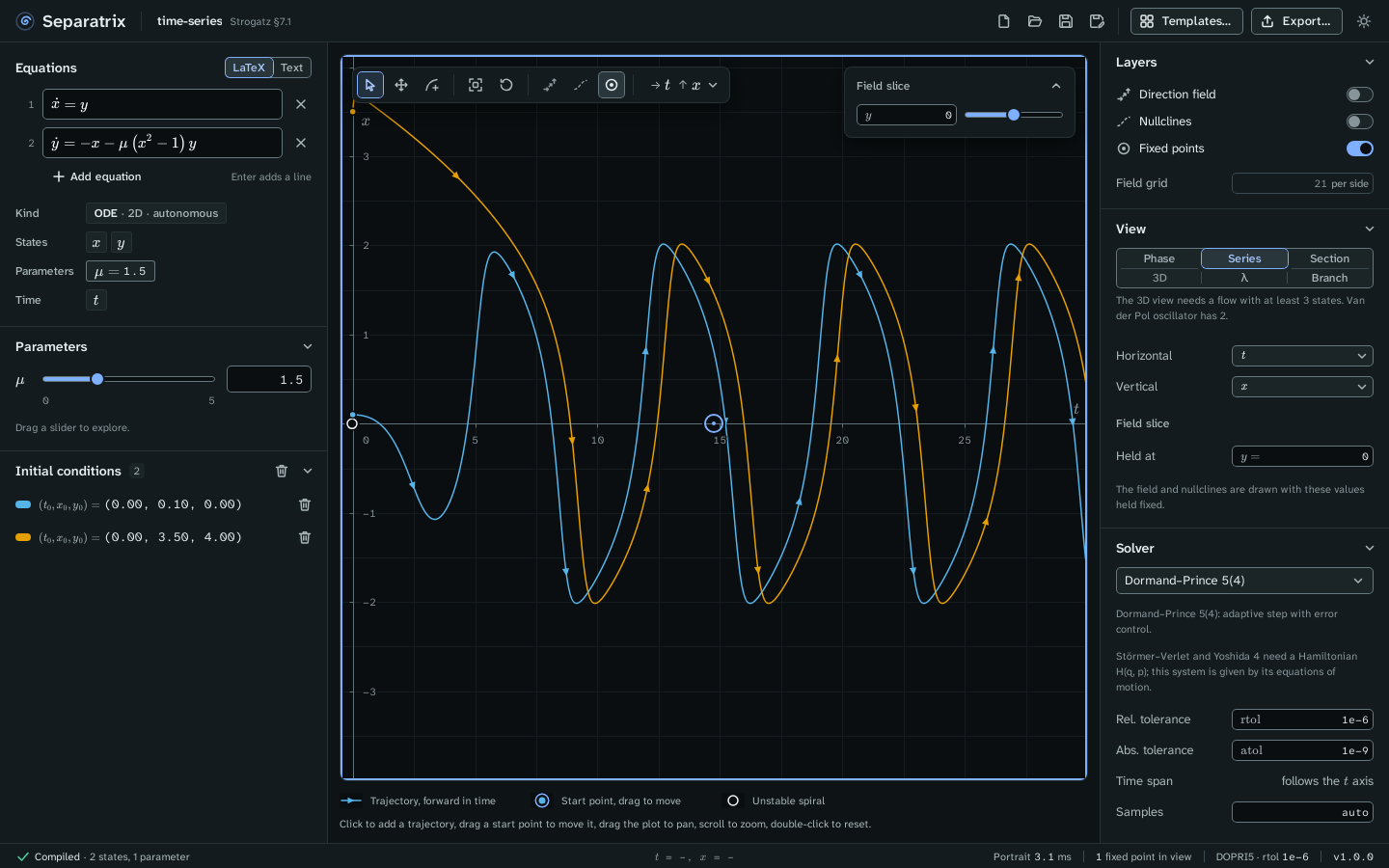
Example project: time-series.sepx, the Van der Pol oscillator of Strogatz §7.1 at μ = 1.5. Both trajectories settle onto the same limit cycle, so after a few periods the two curves differ only by a shift in time.

What the view shows

Series puts time across and the first state up. To plot another state, choose it in the Vertical menu of the View panel or in the axes menu of the plot's toolbar. Either axis can hold time, so you can also put time up and a state across.

In a time series, the time axis sets how far each trajectory runs. The Solver panel's Time span reads "follows the t axis", because the trajectories cover exactly the visible time window. Pan or zoom along t to see more of them.

A one-dimensional flow such as ẋ = sin x (Strogatz §2.1) opens as a time series with its slope field, because a phase plane needs at least two states. The gallery's chapter 2, 3 and 4 examples open this way.

Measure a period

Hover over the plot to read t and x in the status bar. For a sharper number, export the trajectory as CSV (Export figures and data) and measure the period there. For comparison, the Strogatz gate measures the Van der Pol limit cycle at μ = 1 with a period of T = 6.663286, against the book's 6.663287.

Mouse and keys

Click to add a trajectory, drag a start point to move it, drag the plot to pan, scroll to zoom, and double-click to reset. The keys are those of the phase plane, listed in Keyboard shortcuts.